MSP Analysis Tutorial 4: Signal Processing with pfft~
Working in the Frequency Domain
Most digital signal processing of audio occurs in the time domain. As the other MSP tutorials show you, many of the most common processes for manipulating audio consist of varying samples (or groups of samples) in amplitude (ring modulation, waveshaping, distortion) or time (filters and delays). The Fast Fourier Transform (FFT) allows you to translate audio data from the time domain into the frequency domain, where you can directly manipulate the spectrum of a sound (the component frequencies of a slice of audio).
As we have seen in Analysis Tutorial 3, the MSP objects fft~ and ifft~ allow you to transform signals into and out of the frequency domain. The fft~ object takes a group of samples (commonly called a frame) and transforms them into pairs of real and imaginary numbers which contain information about the amplitude and phase of as many frequencies as there are samples in the frame. These are usually referred to as bins or frequency bins. (We will see later that the real and imaginary numbers are not themselves the amplitude and phase, but that the amplitude and phase can be derived from them.) The ifft~ object performs the inverse operation, taking frames of frequency-domain samples and converting them back into a time domain audio signal that you can listen to or process further. The number of samples in the frame is called the FFT size (or sometimes FFT point size). It must be a power of 2 such as 512, 1024 or 2048 (to give a few commonly used values).
We also saw that the fft~ and ifft~ objects work on successive frames of samples without doing any overlapping or cross-fading between them. For practical uses of these objects, we usually need to construct such an overlap and crossfade system around them, as shown at the end of Tutorial 3. There are several reasons for needing to create such a system. In FFT analysis there is always a trade-off between frequency resolution and timing resolution. For example, if your FFT size is 2048 samples long, the FFT analysis gives you 2048 equally-spaced frequency bins from 0 Hz. up to the sampling frequency (only 1024 of these bins are of any use; see Tutorial 3 for details). However, precise timing of events that occur within those 2048 samples will be lost in the analysis, since all temporal changes are lumped together in a single FFT frame. In addition, if you modify the spectral data after the FFT analysis and before the IFFT resynthesis you can no longer guarantee that the time domain signal output by the IFFT will match up in successive frames. If the output time domain vectors don't fit together you will get clicks in your output signal. By using a windowing function, you can compensate for these artifacts by having successive frames cross-fade into each other as they overlap. While this will not compensate for the loss of time resolution, the overlapping of analysis data will help to eliminate the clicks and pops that occur at the edges of an IFFT frame after resynthesis.
However, this approach can often be a challenge to program, and there is also the difficulty of generalizing the patch for multiple combinations of FFT size and overlap. Since the arguments to fft~/ifft~ for FFT frame size and overlap can't be changed, multiple hand-tweaked versions of each subpatch must be created for different situations. For example, a percussive sound would necessitate an analysis with at least four overlaps, while a reasonably static, harmonically rich sound would call for a very large FFT size.
An Introduction to the pfft~ Object
The pfft~ object addresses many of the shortcomings of the basic fft~ and ifft~ objects, allowing you to create and load special ‘spectral subpatches’ that manipulate frequency-domain signal data independently of windowing, overlap and FFT size. A single sub-patch can therefore be suitable for multiple applications. Furthermore, the pfft~ object manages the overlapping of FFT frames, handles the windowing functions for you, and eliminates the redundant mirrored data in the spectrum, making it both more convenient to use and more efficient than the traditional fft~ and ifft~ objects.
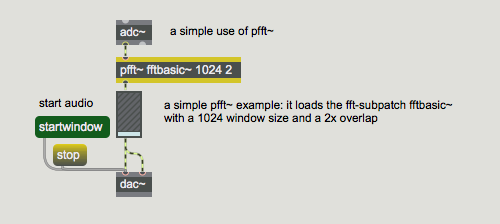
The pfft~ object takes as its argument the name of a specially designed subpatch containing the fftin~ and fftout~ objects (which will be discussed below), a number for the FFT size in samples, and a number for the overlap factor (these must both be integers which are a power of 2):
The pfft~ subpatch referenced above might look something like this:
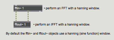
The subpatch shown above takes a signal input, performs an FFT on that signal with a Hanning window (see below), and performs an IFFT on the FFT'd signal, also with a Hanning window. The pfft~ object communicates with its sub-patch using special objects for inlets and outlets. The fftin~ object receives a time-domain signal from its parent patch and transforms it via an FFT into the frequency domain. This time-domain signal has already been converted, by the pfft~ object, into a sequence of frames which overlap in time, and the signal that fftin~ outputs into the spectral subpatch represents the spectrum of each of these incoming frames.
The fftout~ object does the reverse, accepting frequency domain signals, converting them back into a time domain signal, and passing it via an outlet to the parent patch. Both objects take a numbered argument (to specify the inlet or outlet number), and a symbol specifying the window function to use. The available window functions are Hanning (the default if none is specified), Hamming, Blackman, Triangle, and Square. In addition, the symbol can be the name of a buffer~ object which holds a custom windowing function. Different window functions have different bandwidths and stopband depths for each bin of the FFT. A good reference on FFT analysis will help you select a window based on the sound you are trying to analyze and what you want to do with it. We recommend The Computer Music Tutorial by Curtis Roads or The Scientist and Engineer's Guide to Digital Signal Processing by Steven W. Smith. Generally, for musical purposes the default Hanning window works best, as it provides a clean envelope with no amplitude modulation artifacts on output.
There is also a handy window argument to fftin~ and fftout~ which allows the overlapping time-domain frames to and from the pfft~ to be passed directly to and from the subpatch without applying a window function nor performing a Fourier transform. In this case (because the signal vector size of the spectral subpatch is half the FFT size), the time- domain signal is split between the real and imaginary outlets of the fftin~ and fftout~ objects, which may be rather inconvenient when using an overlap of 4 or more. Although the option can be used to send control signal data from the parent patch into the spectral subpatch, it is not recommended for most practical uses of pfft~.
A more complicated pfft~ subpatch might look something like this:
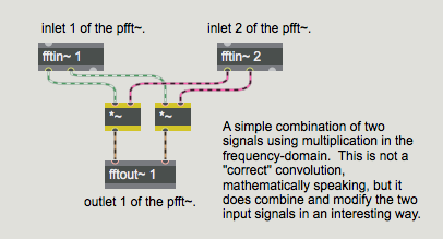
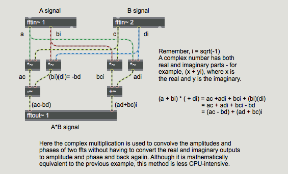
This subpatch takes two signal inputs (which would appear as inlets in the parent pfft~ object), converts them into the frequency domain, multiplies the real signals with one another and multiplies the imaginary signals with one another and outputs the result to an fftout~ object that converts the frequency domain data into a time domain signal. Multiplication in the frequency domain is called convolution, and is the basic signal processing procedure used in cross synthesis (morphing one sound into another). The result of this algorithm is that frequencies from the two analyses which have larger amplitude values will reinforce one another, whereas frequency with weaker amplitude values in one analysis will diminish or cancel the value from the other, whether strong or weak. Frequency content that the two incoming signals share will be retained while frequency content that exists in one signal and not the other will be attenuated or eliminated. This example is not a ‘true’ convolution, however, as the multiplication of complex numbers (see below) is not as straightforward as the multiplication performed in this example. We'll learn a couple ways of making a ‘correct’ convolution patch later in this tutorial.
You have probably already noticed that there are always two signals to connect when connecting fftin~ and fftout~, as well as when processing the spectra in-between them. This is because the FFT algorithm produces complex numbers — numbers that contain a real and an imaginary part. The real part is sent out the leftmost outlet of fftin~, and the imaginary part is sent out its second outlet. The two inlets of fftout~ also correspond to real and imaginary, respectively. The easiest way to understand complex numbers is to think of them as representing a point on a 2-dimensional plane, where the real part represents the X-axis (horizontal distance from zero), and the imaginary part represents the Y-axis (vertical distance from zero). We'll learn more about what we can do with the real and imaginary parts of the complex numbers later on in this tutorial.
The Third Outlet
The fftin~ object has a third outlet that puts out a stream of samples corresponding to the current frequency bin index whose data is being sent out the first two outlets (this is analogous to the third outlet of the fft~ and ifft~ objects discussed in Tutorial 4). For fftin~, this outlet outputs a number from 0 to half the FFT size minus 1. You can convert these values into frequency values (representing the ‘center’ frequency of each bin) by multiplying the signal (called the sync signal) by the base frequency, or fundamental, of the FFT. The fundamental of the FFT is the lowest frequency that the FFT can analyze, and is inversely proportional to the size of the FFT (i.e. larger FFT sizes yield lower base frequencies). The exact fundamental of the FFT can be obtained by dividing the FFT frame size into the sampling rate. The fftinfo~ object, when placed into a pfft~ subpatch, will give you the FFT frame size, the FFT half-frame size (i.e. the number of bins actually used inside the pfft~ subpatch), and the FFT hop size (the number of samples of overlap between the windowed frames). You can use this in conjunction with the dspstate~ object or the adstatus object with the (sampling rate) argument to obtain the base frequency of the FFT:
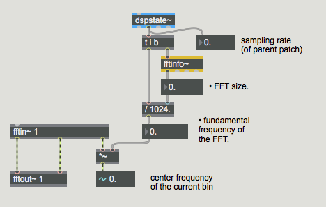
Note that in the above example the number~ object is used for the purposes of demonstration only in this tutorial. When DSP is turned on, the number displayed in the signal number box will not appear to change because the signal number box by default displays the first sample in the signal vector, which in this case will always be 0. To see the center frequency values, you will need to use the capture~ object or record this signal into a buffer~.
Once you know the frequency of the bins being streamed out of fftin~, you can perform operations on the FFT data based on frequency. For example:
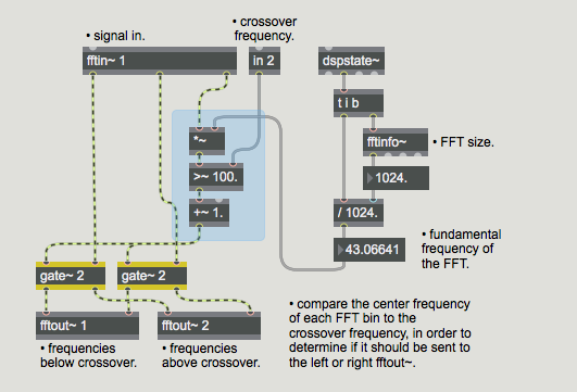
The above pfft~ subpatch, called , takes an input signal and sends the analysis data to one of two fftout~ objects based on a crossover frequency. The crossover frequency is sent to the pfft~ subpatch by using the in object, which passes max messages through from the parent patch via the pfft~ object's right inlet. The center frequency of the current bin — determined by the sync outlet in conjunction with fftinfo~ and dspstate~ as we mentioned above — is compared with the crossover frequency.
The result of this comparison flips a gate~ that sends the FFT data to one of the two fftout~ objects: the part of the spectrum that is lower in pitch than the crossover frequency is sent out the left outlet of the pfft~ and the part that is higher than the crossover frequency is sent out the right. Here is how this subpatcher might be used with pfft~ in a patch
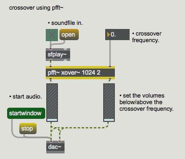
:
Note that we can send integers, floats, and any other Max message to and from a subpatch loaded by pfft~ by using the in and out objects. (See MSP Polyphony Tutorial 1. The poly~ and out~ objects do not function inside a pfft~.)
Working with Amplitude and Phase
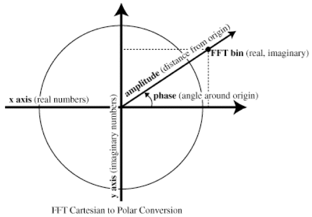
As we have already learned, the first two outlets of fftin~ put out a stream of real and imaginary numbers for the bin response for each sample of the FFT analysis (similarly, fftout~ expects these numbers). These are not the amplitude and phase of each bin, but should be thought of instead as pairs of Cartesian coordinates, where x is the real part and y is the imaginary, representing points on a 2-dimensional plane.
The amplitude and phase of each frequency bin are the polar coordinates of these points, where the distance from the origin is the bin amplitude and the angle around the origin is the bin phase:
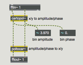
You can easily convert between real/imaginary pairs and amplitude/phase pairs using the objects cartopol~ and poltocar~:
Hanning: FFTsize * 0.25
Hamming: FFTsize * 0.27174
Blackman: FFTsize * 0.21
Triangle: FFTsize * 0.2495
Square: FFTsize * 0.5
So, for example, when using a 512-point FFT with the default Haning window, a full-volume sine wave at half the nyquist frequency will have a value of 128 in the 128th frequency bin (512 * 0.25). The same scenario using a Blackman window will provide us with a value of 107.52 in the 128th frequency bin (512 * 0.21). Even though these are the theoretical maximum values with a single sine wave as input, real-world audio signals will generally have significantly lower values, as the energy in complex waveforms is spread over many frequencies.
The phase values output by the right outlet of cartopol~ will always be between -π and π.
You can use this information to create signal processing routines based on amplitude/phase data. A spectral noise gate would look something like this:
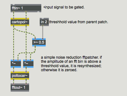
By comparing the amplitude output of cartopol~ with the threshold signal sent into inlet 2 of the pfft~, each bin is either passed or zeroed by the *~ objects. This way only frequency bins that exceed a certain amplitude are retained in the resynthesis (For information on amplitude values inside a spectral subpatch, see the Technical note above.).
Convolution and Cross Sythesis
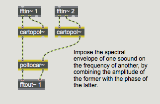
Convolution and cross-synthesis effects commonly use amplitude and phase data for their processing. One of the most basic cross-synthesis effects we could make would use the amplitude spectrum of one sound with the phase spectrum of another. Since the phase spectrum is related to information about the sound's frequency content, this kind of cross synthesis can give us the harmonic content of one sound being ‘played’ by the spectral envelope of another sound. Naturally, the success of this type of effect depends heavily on the choice of the two sounds used.
Here is an example of a spectral subpatch which makes use of cartopol~ and poltocar~ to perform this type of cross-synthesis:
The following subpatch example shows two ways of convolving the amplitude of one input with the amplitude of another:
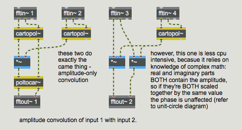
You can readily see on the left-hand side of this subpatch that the amplitude values of the input signals are multiplied together. This reinforces amplitudes which are prominent in both sounds while attenuating those which are not. The phase response of the first signal is unaffected by complex*real multiplication; the phase response of the second signal input is ignored. You will also notice that the right-hand side of the subpatch is mathematically equivalent to the left, even though it uses only one cartopol~ object.
Toward the beginning of this tutorial, we saw an example of the multiplication of two real/imaginary signals to perform a convolution. That example was kept simple for the purposes of explanation but was, in fact, incorrect. If you wondered what a ‘correct’ multiplication of two complex numbers would entail, here is one way to do it:
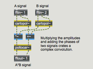
Here's a second and somewhat more clever approach to the same goal:
Time Stretching
Subpatchers created for use with pfft~ can use the full range of MSP objects, including objects that access data stored in a buffer~ object. (Although some objects which were designed to deal with timing issues may not always behave as initially expected when used inside a pfft~.)
The following example records spectral analysis data into two channels of a stereo buffer~ and then allows you to resynthesize the recording at a different speed without changing its original pitch. This is known as time-stretching (or time compression when the sound is speeded up), and has been one of the important uses of the STFT since the 1970s.
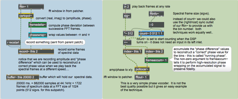
The example subpatcher records spectral data into a buffer~ on the left, and reads data from that buffer~ on the right. In the recording portion of the subpatch you will notice that we don't just record the amplitude and phase as output from cartopol~, but instead use the framedelta~ object to compute the phase difference (sometimes referred to as the phase deviation, or phase derivative). The phase difference is quite simply the difference in phase between equivalent bin locations in successive FFT frames. The output of framedelta~ is then fed into a phasewrap~ object to ensure that the data is properly constrained between -π and π. Messages can be sent to the record~ object from the parent patch via the send object in order to start and stop recording and turn on looping.
In the playback part of the subpatch we use a non-signal inlet to specify the frame number for the resynthesis. This number is multiplied by the spectral frame size and added to the output of a count~ object which counts from 0 to the spectral frame size minus 1 in order to be able to recall each frequency bin in the given frame successively using index~ to read both channels of our buffer~. (We could also have used the sync outlet of the fftin~ object in place of count~, but are using the current method for the sake of visually separating the recording and playback parts of our subpatch, as well as to give an example of how to make use of count~ in the context of a spectral subpatch.) You'll notice that we reconstruct the phase using the frameaccum~ object, which accumulates a ‘running phase’ value by performing the inverse of framedelta~. We need to do this because we might not be reading the analysis frames successively at the original rate in which they were recorded. The signals are then converted back into real and imaginary values for fftout~ by the poltocar~ object.
This is a simple example of what is known as a phase vocoder. Phase vocoders allow you to time-stretch and compress signals independently of their pitch by manipulating FFT data rather than time-domain segments. If you think of each frame of an FFT analysis as a single frame in a film, you can easily see how moving through the individual frames at different rates can change the apparent speed at which things happen. This is more or less what a phase vocoder does.
Note that because pfft~ does window overlapping, the amount of data that can be stored in the buffer~ is dependent on the settings of the pfft~ object. This can make setting the buffer size correctly a rather tricky matter, especially since the spectral frame size (i.e. the signal vector size) inside a pfft~ is half the FFT size indicated as its second argument, and because the spectral subpatch is processing samples at a different rate to its parent patch! If we create a stereo buffer~ with 1000 milliseconds of sample memory, we will have 44100 samples available for our analysis data. If our FFT size is 1024 then each spectral frame will take up 512 samples of our buffer's memory, which amounts to 86 frames of analysis data(44100 / 512 = 86.13). Those 86 frames do not represent one second of sound, however! If we are using 4-times overlap, we are processing one spectral frame every 256 samples, so 86 frames means roughly 22050 samples, or a half second's worth of time with respect to the parent patch. As you can see this all can get rather complicated...
Let's take a look at the parent patch for the above phase vocoder subpatch (called ):
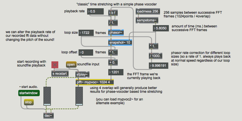
Notice that we're using a phasor~ object with a snapshot~ object in order to generate a ramp specifying the read location inside our subpatch. We could also use a line object, or even a slider, if we wanted to ‘scrub’ our analysis frames by hand. Our main patch allows us to change the playback rate for a loop of our analysis data. We can also specify the loop size and an offset into our collection of analysis frames in order to loop a given section of analysis data at a given playback rate. You'll notice that changing the playback rate does not affect the pitch of the sound, only the speed. You may also notice that at very slow playback rates, certain parts of your sound (usually note attacks, consonants in speech or other percussive sounds) become rather ‘smeared’ and gain an artificial sound quality.
Summary
Using pfft~ to perform spectral-domain signal processing is generally easier and visually clearer than using the traditional fft~ and ifft~ objects, and lets you design patches that can be used at varying FFT sizes and overlaps. There are myriad applications of pfft~ for musical signal processing, including filtering, cross synthesis and time stretching.
See Also
| Name | Description |
|---|---|
| Sound Processing Techniques | Sound Processing Techniques |
| adstatus | Report and control audio driver settings |
| cartopol~ | Signal Cartesian to Polar coordinate conversion |
| dspstate~ | Report current DSP settings |
| fftin~ | Input for a patcher loaded by pfft~ |
| fftout~ | Output for a patcher loaded by pfft~ |
| framedelta~ | Compute phase deviation between successive FFT frames |
| pfft~ | Spectral processing manager for patchers |
| phasewrap~ | Wrap a signal between π and -π |
| poltocar~ | Signal Polar to Cartesian coordinate conversion |