How to enhance object movement
In computer graphics, making objects move according to real-world physical laws is essential for creating believable and immersive scenes. When objects behave as they would in nature—accelerating, slowing down, bouncing, or falling realistically—our brains recognize and connect with that authenticity, making the scene feel more lifelike. By applying principles like inertia, gravity, and friction, you can achieve motion that looks correct and helps the audience engage with the virtual world as if it were real. This adherence to physical laws bridges the gap between digital environments and our physical understanding, enhancing both visual realism and emotional impact.
Let's see how we can improve the movement of objects in Max.
Inertia
Which of the two squares moves "better"?

The blue square seems to have more likeable, believable motion. But why?
Every object in nature has something we call mass—essentially, the “amount of stuff” that makes up an object. Whether it's a tiny pebble or a massive mountain, each one has mass. And with mass comes a natural tendency for objects to either stay put or keep moving in the same way, unless something else (a force) makes them change their behavior. This is a principle known as inertia, part of Newton's first law of motion.
When an object with mass moves from a starting to an ending position, it naturally undergoes acceleration (speeding up) and deceleration (slowing down) due to the forces needed to start and stop motion.
Imagine pushing a car: it doesn't reach full speed instantly but accelerates gradually, as its mass resists sudden changes in motion (because of inertia). Similarly, when you want to stop, the car doesn't halt right away; it decelerates gradually, needing a counterforce (like braking or friction) to slow it down. This process reflects how mass resists both starting and stopping motion, requiring force to change its speed.
How can we give a sense of acceleration and deceleration to the movement of virtual objects? We have three ways to do it:
Physics-based motion
In specific scenarios, it's possible to describe the motion of objects using physical laws. Imagine you have an object with its own mass, and a force attracts it. Given the strength of the force, its direction, and the mass of the object, you can determine the how the object will move as a result of physics.
You can describe the movement of an object with mass subjected to a force using Newton's Second Law of Motion:
where is the object's acceleration. To find the object's position and velocity over time, break this down into discrete time steps and use the following equations.
- Calculate Acceleration: Given the force , find the acceleration of the object as:
- Update Velocity: If you know the object's velocity at time , denoted , update its velocity at the next time step as:
Where is the time interval between steps.
- Update Position: To update the object's position , use the updated velocity:
To summarize:
- calculate Acceleration:
- update velocity:
- update position:
These steps allow you to iteratively compute an object's position and velocity at each time step based on the applied force in the discrete time domain.
When forces are applied to one or more objects in this way, movement becomes an emergent property, naturally incorporating acceleration and deceleration as a result of simulated physics.
This approach to animation is especially useful in particle systems. In these systems, a group of bodies (each with mass) is influenced by one or more forces. The video below demonstrates a simple particle system driven by physically plausible attractors.
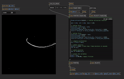
Although this approach to defining motion produces organic and realistic results, it's not always practical or convenient. Movement becomes an emergent property of a "system of rules," which means we don't have direct control over the objects's position in each frame. If precise control over position is required, we need to explore other methods for managing object movement.
"Bend" motion in the temporal domain
To have a better understanding of the problem, let's observe again what's wrong with the yellow square's momevent:

The square moves back and forth without any change in speed. For this kind of movement to happen, it would require infinite acceleration, which could result from either a zero mass or an infinitely strong force. This type of movement is known as linear motion, which is precisely what we aim to avoid.
Linear motion can be desirable if we need to show a "robotic"-like or "digital"---like movement or if you want to describe the movement of a body with marginal mass (e.g., a mosquito).
Let's say we want to move a body from position to in one second. Plotting its linear motion in a graph with time and position on the axis, this is what we get:
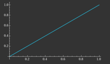
The slope of this line segment represents speed. Here, the object starts at position 0 at time 0, travels steadily, and reaches position 1 at time 1 without any change in speed. However, there should be phases of both acceleration and deceleration for a more natural movement. Beginning with speed = 0, the object should accelerate, then decelerate, and finally stop at position 1, with speed = 0 once more. In technical terms, the slope (or derivative) of the position curve should be 0 at both position 0 and position 1.
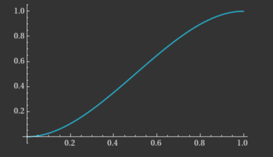
To create such a curve, we can use various mathematical functions that have a derivate of zero at both and . A notable example is the cubic curve:
This happens to be the function plotted in the graph above. This function has all the properties we want in the subdomain [0-1], starting and ending with slope 0. Let's apply this movement path to an object to see the difference.
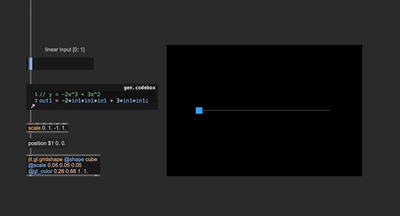
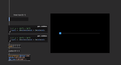
To apply this curve as motion, we simply provide a linear input to the function, which returns a "bent" version.
The function for describing an object's movement doesn't necessarily need to be limited to the subdomain [0-1]. However, it's very convenient to define such a function in this domain because it's easier to perform further manipulations of the motion curve. If you need to express the movement in a range different from [0-1], you can scale the output to the needed range.
From this basic cubic function, you can design many different variations. For example:
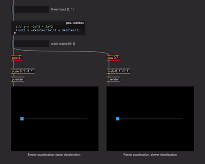
- You can cascade multiple cubic functions to enhance the acceleration and deceleration phases (mimicking a larger mass).
Since the function returns a value within the range [0-1], you can take advantage of this and perform exponentiations to further bend the curve, creating assymetries of the acceleration and deceleration phases while conserving the condition that the slope be zero at and .
Cubic functions are not the only ones with null derivatives at a given subdomain's beginning and end. These are some possible other functions plotted on a graph:
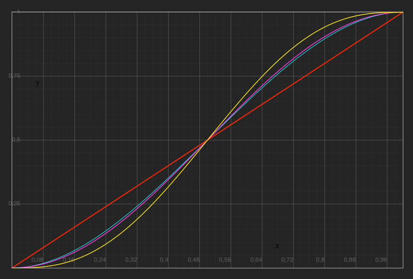
(for reference), , , .
The last one is a quintic function, and it's particularly noteworthy because it not only has zero first derivatives at and but also zero second derivatives at and . This is relevant for us because the first derivative of the motion function represents speed (the function's slope), while the second derivative represents acceleration (the slope of the speed function). Functions like the cubic one we used earlier show a discontinuity of the second derivative (acceleration). Although visually better than linear functions to describe motion, an infinite force or a null mass is still required to make a body accelerate like that.
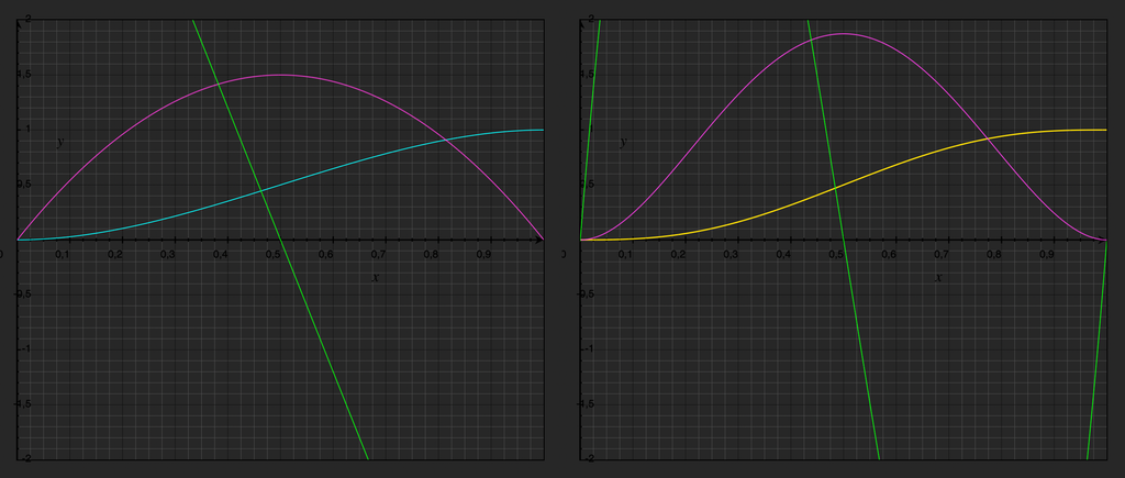
Left: , , ; right: , , ;
You can see that the second derivative (in green) of the cubic function is a straight line, and it's non-zero at and . In the quintic function case, it touches the abscissa at both and .
If we want to describe a motion function like "the cool kids", we can opt for such a quintic function.
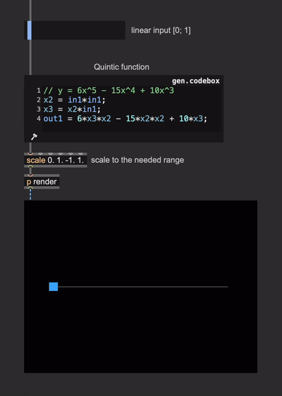
When do these functions come in handy? In the previous section, we described motion as the result of forces acting on bodies with mass. Because of this, we didn't have precise control over where and when a body moves. Using motion functions is essentially the reverse approach: You can define the exact initial and ending positions and how long the object takes to complete the movement, but you don't control the precise acceleration at any point along the object's path (Having said that, you can of course derive which forces are implied in the motion for a known object mass to make it move along the curve you define).
This kind of control over object movement is very useful when you must express an initial or ending position and define how long it takes to complete the movement. One pefect example scenario would be transition effects.
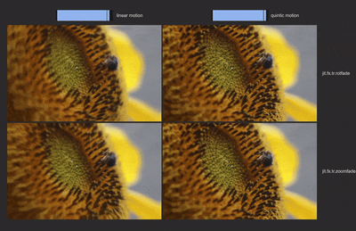
The transitions on the left look "mechanical", while the two on the right appear fluent and more "natural".
If you need to create motion curves for multidimensional movement (e.g., an object moving in a 3D space), you can apply the same principles to each dimension.
The strength of this approach is precision over time. Things start and stop moving exactly when we want to. Still, this method becomes unpractical if we need to define complex movement over time. We could "glue" together pieces of functions to describe a complex motion, but if we do so, we also have to guarantee the condition of continuity for the first (and eventually second) derivative. While this is not impossible (we could solve systems of equations to compute ad-hoc pieces of functions), it may be inconvenient. It's better to approach the problem from a different perspective for such a scenario.
Filter motion in the frequency domain
Any variable phenomenon, like the changing position of an object in space, can be broken down into a series of simpler waves—sines and cosines! This idea comes from something called the Fourier series, and it's a powerful way to represent complex, varying signals.
By adding up these waves correctly, we can reconstruct any complex movement or signal. Each sine or cosine wave in the series has a specific frequency, amplitude (height), and phase (shift), which together help us "build" the final pattern. This method is like having a toolkit of building blocks that, when put together, mimic the movement or variation we want to describe.
The beauty of this approach is that it applies to virtually anything that changes over time or space, whether it's the flicker of light, the beat of a drum, or an object's motion. Fourier series essentially gives us a “recipe” for recreating any variable pattern with an infinite sum of these simple wave-like functions.
Let's look at our yellow square motion from a different perspective, borrowing some tools from MSP-land:


We intentionally removed all numerical references from the signal objects, for example the scaling and FFT size for spectroscope~. These audio objects are being used for a visual demonstration, so their precise numerical configuration, which depends for example on the Max's sample rate, would be a distraction. Therefore, signal-rate objects are shown here without revealing "the numbers".
The two graphs above show the square's motion function from two different perspectives:
- Left: the position moving linearly from the beginning to the end of the motion path.
- Right: the spectral decomposition of the motion function on the left.
By "breaking" the motion function into a combination of sine waves using a Fourier analysis, we can see that multiple elementary waves of increasing frequency and decreasing amplitude are required to give rise to the "triangular" motion our square is going through.
Actually, to combine into a perfect triangular path, an infinite amount of sine waves is needed.
What we're intrested in is what happens to our motion function if we filter out some of the highest sine waves. To perform filtering, since we are using signal-rate objects, we can use a simple audio low pass filter.
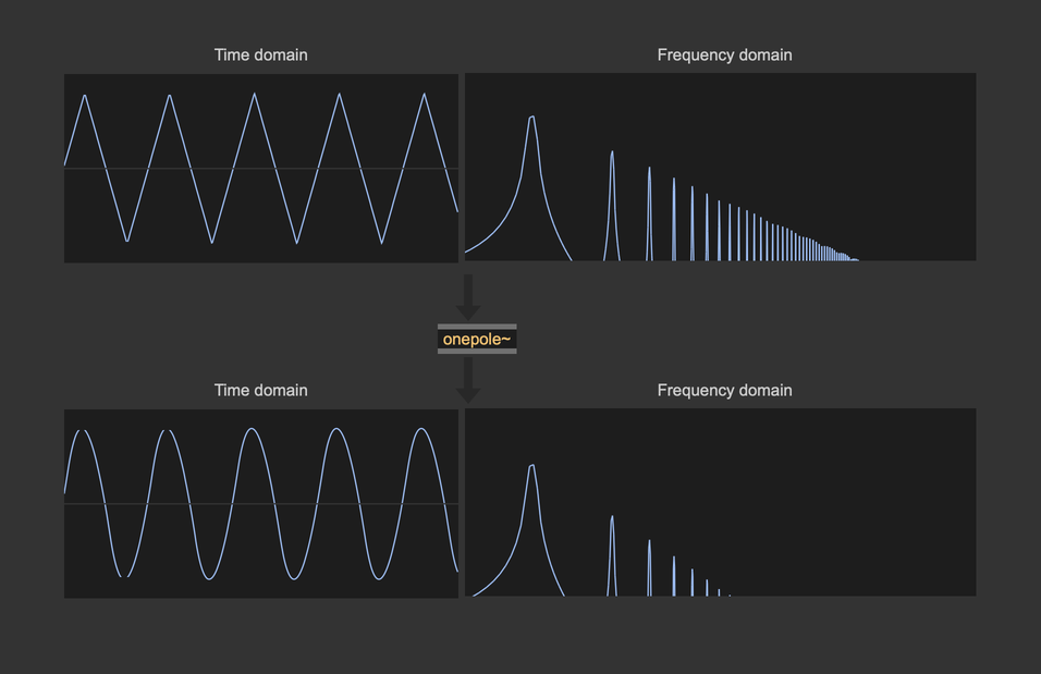
The low-pass filter attenuates high frequencies, and you can see that after filtering, the motion function on the left has been rounded off. Simply by filtering, we've created juicy acceleration and deceleration phases! Controlling the low-pass filter cutoff, we can control the motion path roundness, mimicking a variation of the object's mass. This brings us to another way we can use to define non-linear motion:
You can create a straightforward linear motion path (simple to define and control), interpret it in the frequency domain, and filter out the high frequencies. This process results in a smoother motion that naturally incorporates acceleration, deceleration, and inertia.
The filters described in the following section are infinite impulse response (IIR) filters that work in the time domain. When we say "operate in the frequency domain," we're not implying any spectral processing; rather, we're describing how the filters reduce the amplitude of certain frequency ranges.
Let's bring this concept back to Jitterland and see how we can use it to improve object motion.
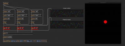
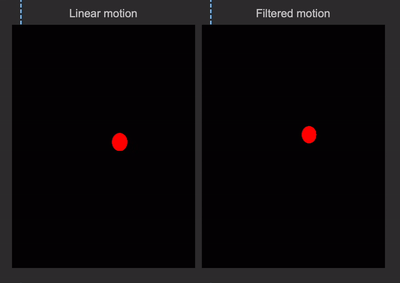
Here's a simple scene with a red sphere that moves randomly across the screen. The motion is smoothed with a low-pass filter using the slide object. The two graphs on the right show the unfiltered and filtered motions. Overall, the filtered movement looks realistic, with the sphere experiencing acceleration and deceleration. Here's a side-by-side comparison of the unfiltered vs. filtered motion:
The slide object is a possible choice for filtering, but it's not the only one. Max offers a variety of low-pass implementations for audio signals, but there are few built-in options for filtering streams of messages, matrices, and textures. Still, we can build our filters from scratch. Let's see a couple of practical low-pass implementations for us, Jitterheads.
Digital filters can be tricky to navigate, and designing them is a complex subject that deserves its own in-depth discussion. For this article, we'll demonstrate some filter implementations without diving deeply into technical details. Instead, we'll provide qualitative insights and examples of when and how to use these filters, keeping things accessible and practical. (Plus, I'm personnaly not a filter design expert!)
One-pole filter
This is the simplest possible low-pass filter:
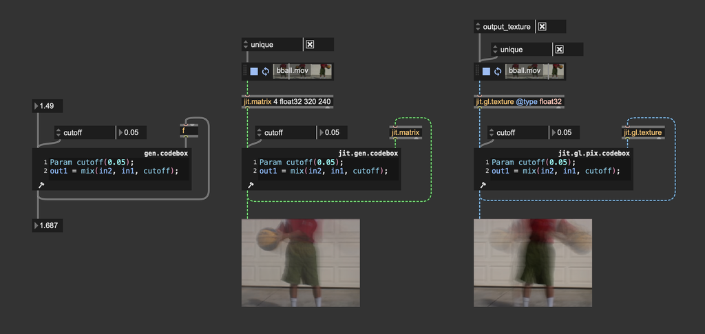
This low-pass filter, though simple, can be very effective. It works by averaging values from the current frame with values filtered from previous frames. Depending on how your position data is represented, you can customize a one-pole filter to smooth data like messages, matrices, or textures. The filter's strength is controlled by an interpolation value (ranging from 0 to 1), which determines how much weight the current frame has versus the previous frame.
Since one-pole filters are 1st-order filters, they provide a gentle frequency cut of 6 dB per octave, resulting in smooth filtering. To make the filter more selective, you can increase the order by cascading multiple one-pole filters. Each additional filter in the chain increases the overall filtering order by 1.
One-pole low-pass filters can be implemented in various ways, including using some built-in objects. Here we implemented it in a gen codebox to give a clearer view of the algorithm's inner workings.
Biquadratic filters and Butterworth filters
A filter can be constructed (in the case of an analog filter) or implemented (if digital) in various ways. A filter topology refers to the structural arrangement or configuration used to implement a filter in electronics or digital signal processing. The topology defines how components (such as capacitors, resistors, and inductors in analog filters, or coefficients and delays in digital filters) are organized and interconnected to achieve the desired filtering effect.
In the world of digital filters, a widely used filter topology is biquadratic filters (or biquad filter for short). These kinds of filters are appreciated for their flexibility, as they can be used to implement different filter responses (low-pass, high-pass, band-pass, etc.).
Biquad filters rely on specific coefficients to control their operation. These coefficients allow you to decide which frequencies are boosted or reduced and determine the filter's type. A biquad filter operates using a formula with five principal coefficients: , , , , .
In practical terms, the filter equation looks like this:
- is the output signal at the current sample.
- , , and are the current and past input samples.
- and are the past two output samples.
And a Maxy implementation of such a filter topology looks like this:
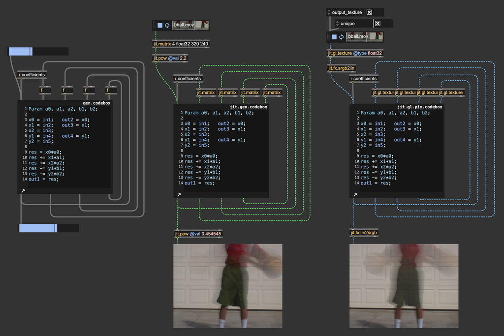
The objects biquad~ and jit.fx.ti.filter implement biquad temporal filters like the ones displayed above.
How can we compute the correct filter coefficients to get the desired filter response? Each kind of filter has its onw coefficient calculation.
Check out the patch "gen~.biquad.maxpat" for looking at various biquad coefficient computations:
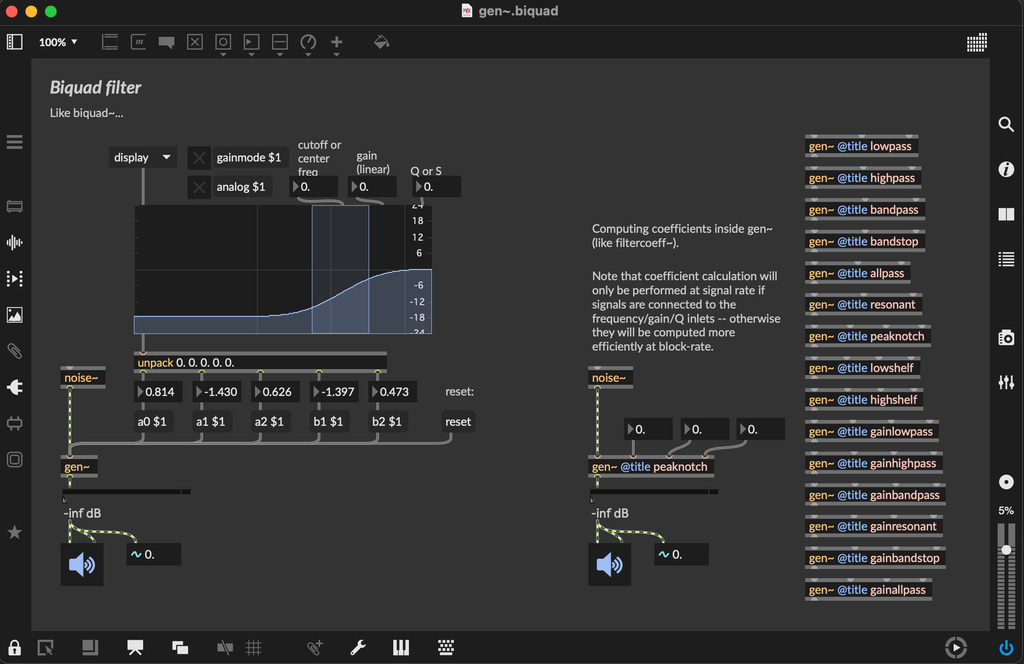
For our goal, there's a specific filter response we're particularly interested in: low-pass Butterworth filters. Butterworth filters are a type of signal filter known for their maximally flat frequency response in the passband, meaning they allow frequencies up to a specified cutoff to pass through without significant attenuation or ripples. This makes Butterworth filters ideal when smooth, distortion-free filtering is needed. The transition from passband to stopband (attenuation region) is gradual compared to other filters, like Chebyshev or elliptic filters, which prioritize sharper cutoffs at the expense of flatness. Moreover, Butterworth filters generally offer a near-linear phase response, especially at lower frequencies, which minimizes phase distortion for signals passing through the filter. In other words, butterworth filters are designed to be as transparent as possible regarding the filtered signal.
We can implement a digital Butterworth filter response using a biquad filter. Let's see how to compute proper coefficients for this kind of filter.
Define Parameters:
- Cutoff frequency (in Hz) – the frequency at which the filter starts attenuating the signal.
- Sampling rate (in Hz) – the rate at which the signal is sampled. In our case, the video frame rate.
The cutoff frequency (in the digital domain) needs to be pre-warped using the following formula:
Where is the angular frequency. The warped frequency is then:
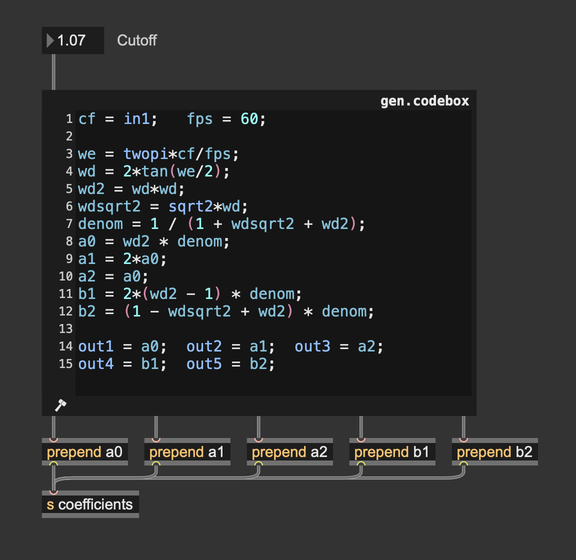
The coefficients for a 2nd-order low-pass Butterworth filter are calculated as follows:
This is the coefficient computation implemented in Max:
Enough math, let's see how this filter looks! Here's a straightforward test patch where the colors of an input video are interpreted as 3D positions for a particle system. In particular, particles are distributed evenly across the horizontal dimension, and we use the color luminance to determine vertical positioning.
The rendering looks "ok," but let's try to filter out the particle movement.
The particles look way more lively! Let's now try using higher-order Butterworth filters. Here, we cascade four filters to get 8th-order filtering. We also decreased the cutoff value a little because we don't need to roll it down so much to attenuate high frequencies with such a high-order filter.
The particle movement became "bouncier"! Before reaching the input position, each particle oscillates slightly. Cascading even more 2nd-order filters, the bouncing effect becomes more pronounced. We can even try to "trigger" a new particle arrangement and look at how the filter smoothens out motion:
As you can see, decreasing the cutoff value resembles a mass increase. Since we have our Butterworth coefficients calculator exposed, we can go a step further and assign different cutoff values to each particle. I slightly reworked the coefficients calculator and the biquad filter to read from matrices the coefficient values.
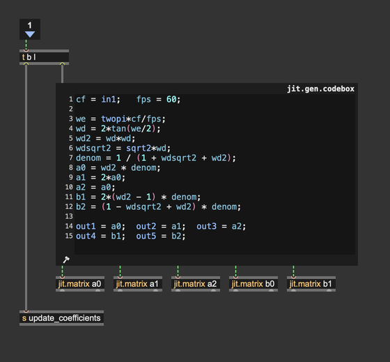
The coefficient calculator has been turned into a jit.gen.codebox to operate on matrices, but the code stays the same.
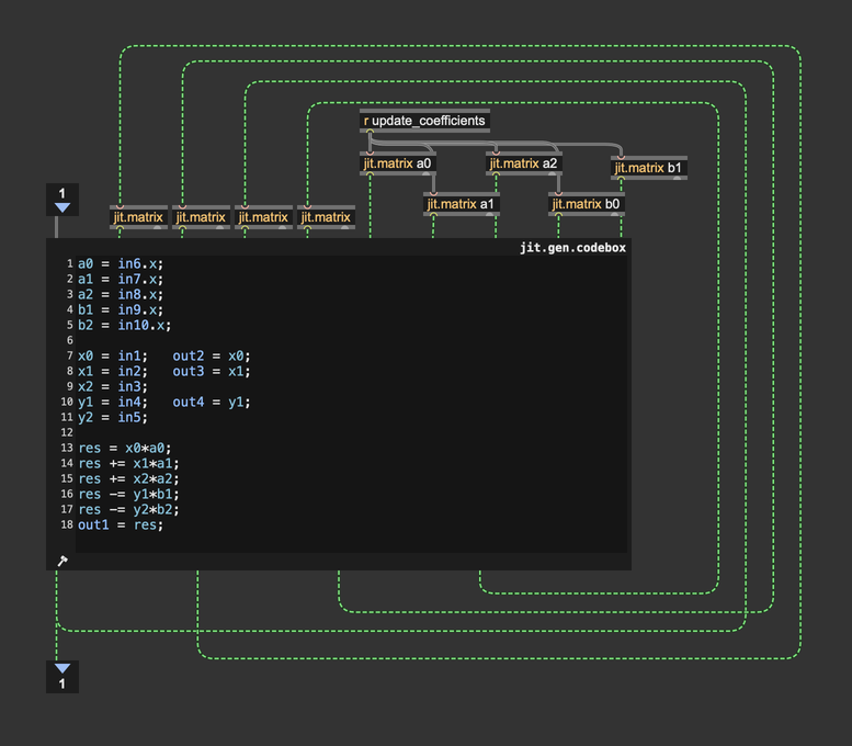
And in the biquad computation, coefficients are no longer provided as params but as matrices.
With control over individual cutoff values, you can differentiate the object's behavior. In the patch below, I had fun generating random cutoff values (in the range [2-4]), and then I tried to assign progressively increasing cutoff values (from left to right). With this degree of control, you can create very interesting animations.
Filters are an excellent tool for enhancing the appearance of complex object motion, with Butterworth filters being especially well-suited for this purpose. Much like motion functions, filters allow you to smooth a motion path by providing a linear motion as input, producing results that naturally reflect physically plausible behavior. However, this approach to motion smoothing has a limitation: filters tend to introduce a slight delay in timing, reducing temporal precision. In the end, there's no single best approach—each situation calls for the right tool to achieve the desired effect.
It's worth highlighting that Max provides a set of objects specifically crafted to simplify object motion management: jit.anim.drive, jit.anim.path, and jit.anim.node. These objects are ideal for high-level motion control, as they can be adjusted through intuitive, meaningful parameters. Additionally, a set of external objects called “ease” provides tools for defining motion functions without needing to dive deeply into the underlying math. Max, as always, is a highly modular, multi-level programming environment, allowing you to find solutions that best suit your needs.
Motion blur
Oh, no! Moving squares, AGAIN?!?!1! This is the last time, I swear... So, which one moves "better" ?

You should know it by now... the blu one always wins.
Both squares are going under the same (quintic) motion, but the rendering of the blu square incorporates motion blur.
Motion blur is a visual effect that simulates the natural blurring of moving objects, making animations and videos look more realistic. When you take a photo of a fast-moving car, and it appears slightly blurred along its path, that's motion blur at work! This happens in real life because, during the time it takes to capture the image, the car moves, creating a streak or blur along its direction of motion.
We can replicate this effect to give the impression of speed and smoothness. Motion blur can enhance the realism of fast-paced scenes by blurring objects in the direction of motion, making them look less "stiff" or "choppy." Let's break down the real-world phenomena that lead to motion blur:
Motion blur arises in photography when there is relative motion between the camera sensor and the subject during the exposure time. Exposure time, also known as shutter speed, is the time during which a camera's sensor (or film) is exposed to light. During this time, the camera's shutter is open, allowing light to reach the sensor and create an image. In 3D rendering, time is discretized into frames, which are "undivisible" time units. In such a context, we can think of exposure time as the intra-frame time (the time elapsed between one frame and the next). When rendering a scene, objects appear istantaneously on screen at each frame, and there's not an intermediate phase in which the virtual camera is exposed to light, hence no motion blur is rendered. If we want to add this effect to our images, we have to make it ourself.
There are several methods to create a motion blur effect, and the choice of which to use depends on the rendering method we're using, the time budget we have for rendering a frame, and the kind of rendered scene. Here's a list of some approaches to motion blur rendering:
Ray-traced motion blur
This sounds fancy, but in reality is the simplest way to create blurry motions as it replicates the phenomena that produce the blur in the real world. If you're rendering your scene using a ray-based method (e.g., ray marching or path tracing) you assign meaningful colors to the pixels by "shooting" rays from the camera point of view into the scene, finding the intersections of each ray with the surrounding geometry, and computing light transport to shade the pixels. This process is repeated multiple times per frame, gathering numerous samples from the scene and averaging their color contributions. If you move the objects in the scene or the camera itself while collecting color samples, it's like having motion during the exposure time. As result, the rendered images will naturally account for motion blur.
This guide is not about implementing ray-tracing rendering solutions, but since it's feasible with standard Max and custom shaders, we include this method to give the reader a broader perspective on the topic.
Motion blur by accumulation
We said that in digital rendering images "appear" istantaneously at each frame. Consider an object at frame to be in position which was in position at the previous frame . When rendering frames and in succesion, the object appears as jumping from to . If all we can do is to render an object in a single specific position at each frame, we could recreate the effect of a motion trail by rendering multiple objects covering a set of positions between and .
Motion blur through accumulation consists of rendering the same object multiple times filling the space between and through a "gradient" of intermediary positions.
Let's set it up in Max:
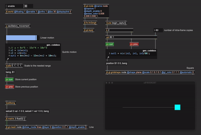
In the left-top corner of the patch, we're generating a motion path, and at each frame we store the current and the previous (horizontal) postions into the pv objects labeled "curr" and "prev". The right side is where the accumulation takes place. There's a square drawn with the object jit.gl.gridshape, which is set to @automatic 0, meaning it doesn't render automatically to screen at each frame, but only when it receives a bang message (or a "draw" message). The jit.gl.gridshape object has been bound to a jit.gl.node object which is rendering to a texture through the attribute @capture 1. A nice thing about jit.gl.node is that it reports from the right-most outlet when the capturing phase begins via "begin_capture" messages. When the capturing phase begins, it triggers the drawing of multiple copies of the square. In the patch an uzi object triggers 80 iterations of the drawing process. At each iteration, the previous and the current positions are linearly interpolated and a square is drawn at the resulting position.
uzi is set to count from 1 to 80, and in the interpolation process we divided the iteration index by 80. This means that the interpolation factor for the function "mix" goes from 0.0125 up to 1. We're intentionally avoiding an interpolation factor of 0 so as not to re-draw a square at the exact previous position. The difference is visually unnoticeable, but it's more conceptually consitent.
The patch succesfully draws 80 progressively shifting copies of the square, but the result doesn't look like a proper blur—it's more like an expanding rectangular block. That is because we're violating the laws of energy conservation. We won't end up in jail for that, but we surely must account for it.
Think again at the real world example where a camera takes a picture of a moving object. The light reaching the camera sensor is the same light that bounced off the subject of our picture towards the camera. If the subject is moving or still, the amount of energy (light) hitting the camera sensor must be the same. In our example, we're drawing 80 copies of the square without changing the amount of light they reflect towards the digital camera, meaning that we're increasing the emitted light intensity by a factor of 80. To fix it, we have to divide the amount of emitted radiance of each copy by , where is the number of copies, so that the total amount of emitted light sums up to 1. In other words, we have to compute an average.
Now, we're not rendering each square to a separate texture; if that was the case, we could have performed a running average over the rendered textures. What we're doing is rendering the copies of the square to the same render target. Therefore, if we want to compute an average (sum and divide by ), we must do it at the rendering stage.
With that in mind, this is how our patch looks now:

We enabled jit.gl.gridshape's color blending via @blend_enable 1 and disabled depth testing with @depth_enable 0. The blending mode attribute @blend has been set to "add", because if we need to perform an average computation, we must sum the colors of each square. Prior to rendering, the square's color intensity has been divided by the number of copies.
This "time interpolation" process must be applied to any parameter that influences positioning, such as scaling and rotation.
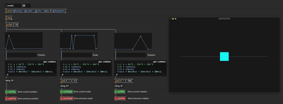
Here is a short sequence for position, scaling, and rotation using linear piece-wise functions passed through our "quintic bender". The patch stores both the values at the current frame and at the previous frame for later interpolation. To let scaling and rotation create motion blur, the right half of the patch now looks like this:
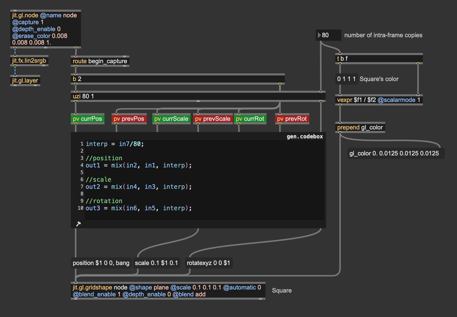
Rotation and scaling go through the same treatment as position values.
In the patch, we explicitly store position, rotation, and scaling for later manual interpolation. Another approach would be to store the current and previous states of jit.gl.gridshape as presets and interpolate between them using Max built-in tools.
To make a fair comparison, this is the same scene rendered without and with motion blur:

The animation looks smoother overall, and we perceive the motion's speed and direction better, particularly when the shape moves fast.
You may have noticed that we're rendering the scene at 30 fps (jit.world's @fps 30.). Motion blur is about capturing the intra-frame movement, and the longer the exposure time, the more evident the blur. To increase the exposure time you should use low @fps values, as .
The number of frames per seconds influences the animation's overall look. Very low frame rates (from 10 to 20 fps) will make you video look like a hand-draw cartoon (especially when motion blur is disabled), low frame rates (from 24 to 30 fps) produce a cinematic look, and higher frame rates (40 - 60 fps) result in videogame-like animation.
Now that we have the basic setup for applying motion blur, let's have fun with a larger-scale scene. Here I recreated one of the most iconic effects ever: the Rutt-Etra video synthesizer. I'm distributing some lines on a plane and determining the height of the lines using the luminance from a video.
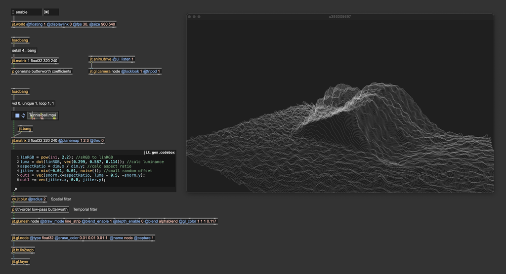
The render looks like this:
And with motion blur enabled:
Video compression is not helping in showing the difference, but it can be better grasped with a side-by-side still image:

Let's see how to add motion blur in this context. The lines' position is no longer determined by a single @position parameter; instead, we store the position of the vertices using matrices. Therefore, to store the current and previous positions, we can use use jit.matrix instead of pv.
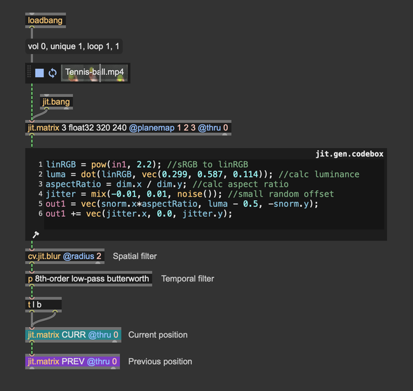
And this is how I'm managing the accumulation process.
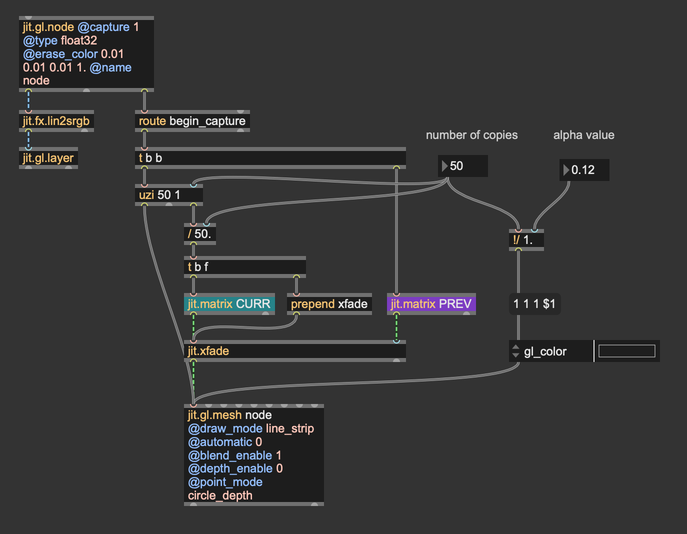
The linear interpolation between the set of current postitions and the set of previous positions is computed with the object jit.xfade. To set the desired transparency for the lines, the alpha component of the line color is divided by the total number of copies. You can disable motion blur by setting the number of copies to 1 (only the current set of positions gets rendered).
I like the result, but there's still something we're not considering; let's try to stop the video player and let's move the camera around.
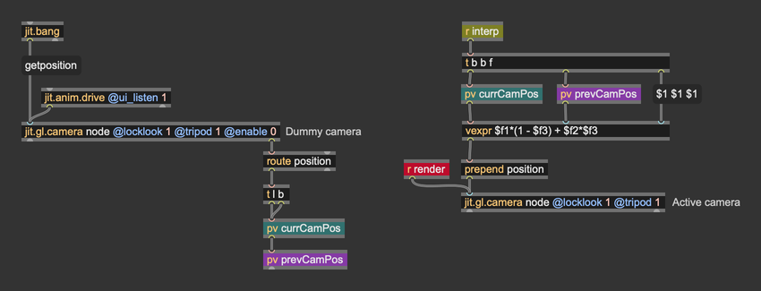
The camera movement doesn't produce any blur. As we said at the beginning, motion blur arises when there's a relative motion between the camera and the objects in the scene. Hence, we have to consider the camera motion as well. To make it happen, we almost have all we need already. The geometry is rendered multiple times in each frame (50 times in the above patch), so we need to temporally interpolate the intra-frame camera movement and render each copy of the geometry as seen from different camera positions.
For a clearer implementation, I re-designed the acculumation process using wireless connections:
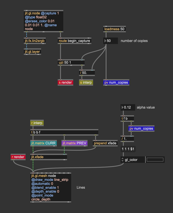
Interpolating camera positions can be somewhat complex. To move the camera using jit.anim.drive, two jit.gl.camera objects are required. The first camera, referred to as the "dummy" camera in the patch, is controlled by jit.anim.drive and provides its current position as well as its previous position. These positions are queried from the dummy camera and stored in two pv objects. The second camera is used for rendering, interpolating linearly the current and previous positions.
Finally, also the camera movement incorporates motion blur:
In the examples above the intra-frame motion is computed by interpolating linearly between the current position () and the previous position (). This means that the intra-frame motion is slways a straight line. For fast movements with frequent changes in direction, it may be worth using different forms of interpolation capable of producing curved paths (e.g., cubic spline interpolation), at the cost of longer history of position values required.
Motion blur by accumulation is a powerful method to create a blur effect along the direction of an object's motion. However, it comes with some challenges:
High Computational Cost
This technique requires rendering multiple copies of the geometry, which can be resource intensive, especially for real-time applications. Reducing the number of copies is an option, but it often results in visible artifacts. The blur may appear discontinuous, and individual geometry copies may become discernible, forming regular, unwanted patterns. If you need to reduce the number of copies, consider these strategies:
- Add Randomness: Instead of regular sampling, try quasi-random sequences, such as Halton sequences or blue noise, for temporal interpolation. This introduces randomness that helps mask the low number of copies. Our brains are excellent at detecting patterns, so replacing regularity with randomness can effectively smooth the motion blur (a Monte Carlo-inspired approach).
- Adaptive Copy Count: Adjust the number of copies based on the displacement between frames. For example: If a geometry remains stationary between frames, a single copy suffices since no motion blur is needed. For geometries with significant displacement between frames, increase the number of copies to adequately cover the motion path. This approach requires computing the displacement for each point (e.g., from position to ) and setting the copy count accordingly. Additionally, adjust the object's color to maintain energy conservation, ensuring the blur effect remains visually consistent.
All the patches shown in this paragraph operate on positional data stored and processed by the CPU. For faster execution times, it's possible to replicate the accumulation process on the GPU, using jit.gl.buffer or jit.gl.texture instead of matrices, and using custom geometry shaders or GPU instancing for drawing the geometry.
Transparency Requirement
This method relies on blending during the rendering stage, making it suitable only for semi-transparent objects. This introduces complications with rendering order and depth sorting, as transparent objects often require careful handling to avoid visual artifacts.
Practical Usage
Due to these constraints, motion blur by accumulation is typically applied to simple geometries like points and lines. For more complex geometries, alternative techniques may be more suitable. If you need to blur complex objects, consider other methods that circumvent these limitations.
Motion blur as post-processing effect
Motion blur as a post-processing effect is a technique used in computer graphics to simulate the visual blur that occurs when objects or the camera move quickly during a scene. Unlike geometry-based motion blur, which involves modifying or duplicating the geometry during rendering, post-processing motion blur is applied as an image-based effect after the main rendering process is complete. A motion blur effect can be implemented following these steps:
- Render the scene as usual.
- Render motion vectors for each pixels. Motion vectors are mathematical representations of the movement of pixels or objects between consecutive frames in a video or rendered scene. They describe the direction and magnitude of movement in screen space. In Max you can render motion vectors by setting the @capture attribute of jit.gl.node to the value 3. This will make jit.gl.node render to 3 distinct render targets (textures), and the third one will contain motion vectors, encoded as red = horizontal movement, and green = vertical movement.
- Make the blur: the motion vectors are used to determine the direction and intensity of the blur for each pixel. Using the motion vectors, neighboring pixels are sampled along the direction of motion to create a streaking or smearing effect.
- Composite: the blurred pixels are combined with the original image to produce the final frame, giving the illusion of motion blur.
Some advanced motion blur effects may need additional steps, like rendering the distance of each pixel from the camera (depth).
In max you can implement this process yourself, using custom shaders, or you can use jit.gl.pass @fxname motionblur. This effect implements a motion blur filter using the steps described above. As long as all objects in the scene are shaded by either jit.gl.material or jit.gl.pbr, this pass FX will produce a blur when the objects or the camera move.
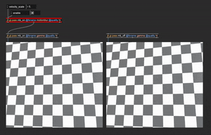
This effect has a single control, @velocity_scale, which determines the amount of blur to apply in the direction of motion.
Post-processing motion blur effects are widely used, because they're not as demanding as the accumulation approach in terms of computational resources. Additionally, the amount of blur is independent of the frame rate: you can simulate the motion blur of a low frame rate even when rendering at a high frame rate. This makes it possible to achieve a "cinematic look" in high frame rate renders. This feature, combined with its efficiency, makes this approach to motion blur particularly well-suited for video games and graphics applications that demand high responsiveness. Still, motion blur as post-processing effect has one major disadvantage: the motion blur effect is limited to the confines of the object itself.
When an object moves, the motion blur appears accurate only within the boundaries of its original shape. This limitation arises because motion vectors, which guide the direction and intensity of the blur, are inherently tied to the object's silhouette. As a result, the blur cannot extend beyond the object's outline.
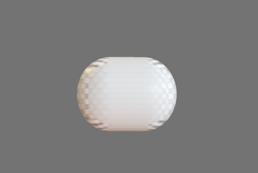
Various techniques have been developed to address this limitation, such as deforming the geometry in the direction of motion or "inflating motion vectors." The latter involves extending the motion vectors beyond the object's original boundaries, allowing the blur to extend past the shape's silhouette. While these methods help mitigate the issue, they can introduce new challenges. For instance, a stationary background object might appear blurred even if it isn't moving. Currently, these methods are not implemented in Max due to their highly context-specific nature. However, I encourage you to explore and experiment with these approaches by creating custom shaders.
Conclusion
This concludes our in-depth look at some of tools we can use to improve the motion of objects on screen. There is no universally correct or incorrect way to utilize the tools and techniques discussed. Each method serves as a creative option in your toolbox, and the decision on which to use should be guided by your artistic intent, the performance limitations of your hardware, and the specific message or mood you wish to convey through your rendering. Whether prioritizing realism, stylization, or efficiency, the power lies in your ability to adapt these tools to meet the unique needs of your project and bring your vision to life.
In summary
- Replicating how objects move in the physical world can help scenes feel more realistic.
- Consider describing motion through forces and masses if you don't need precise control over positioning and timing.
- Describe movement thought motion functions if you need precise control over when and where movement starts and stops; quintic functions are well suited for the task as they replicate physically-plausible acceleration and deceleration.
- Use temporal filters to smooth out complex motion; low-pass butterworth filters can produce pleasent and beliveable movements.
- Motion blur is the physical phenomenon that arises when objects move while cameras take photos; digitally replicating this effect can help convey a better perception of movement and lead to more realistic renderings.
- Motion blur by accumulation produces very good results, but it's demanding of computing resources, and typically suitable for simple geometries, like points and lines.
- Motion blur as post-processing effect is preferred in complex scenes, as it's not as demanding as the accumulation approach. You can incorporate it in your scenes via jit.gl.pass
@fxname motionblur.