MSP Analysis Tutorial 3: Using the FFT

This tutorial references the patcher 03aFourierAnalysis.maxpat

Fourier's theorem

The French mathematician Joseph Fourier demonstrated that any periodic wave can be expressed as the sum of harmonically related sinusoids, each with its own amplitude and phase. Given a digital representation of a periodic wave, one can employ a formula known as the discrete Fourier transform (DFT) to calculate the frequency, phase, and amplitude of its sinusoidal components. Essentially, the DFT transforms a time-domain representation of a sound wave into a frequency- domain spectrum. This spectrum can also be transformed back into a time-domain waveform.

Typically the Fourier transform is used on a small ‘slice’ of time, which ideally is equal to exactly one cycle of the wave being analyzed. To perform this operation on ‘real world’ sounds -- which are almost invariably not strictly periodic, and which may be of unknown frequency -- one can perform the DFT on consecutive time slices to get a sense of how the spectrum changes over time.

If the number of digital samples in each time slice (or frame) is a power of 2, one can use a faster version of the DFT known as the fast Fourier transform (FFT). The formula for the FFT is encapsulated in the fft~ object. The mathematics of the Fourier transform are well beyond the scope of this manual, but this tutorial chapter will demonstrate how to use the fft~ object for signal analysis and resynthesis.

Spectrum of a signal: fft~

fft~ receives a signal in its inlet. For each slice of time it receives (512 samples long by default) it sends out a signal of the same length listing the amount of energy in each frequency region. The signal that comes out of fft~ is not anything you're likely to want to listen to. Rather, it's a list of relative amplitudes of 512 different frequency bands in the received signal. This ‘list’ happens to be exactly the same length as the samples received in each time slice, so it comes out at the same rate as the signal comes in. The signal coming out of fft~ is a frequency-domain analysis of the samples it received in the previous time slice.

Actually, the analysis produced by fft~ is two parallel signals. That's because the math involved produces complex numbers, which have a real and imaginary component. The real components are output from the left outlet and the imaginary components from the middle. Both signals are required for spectral processing.

Although the transform comes out of fft~ in the form of a signal, it is not a time-domain signal. The only object that ‘understands’ this special signal is the ifft~ object, which performs an inverse FFT on the spectrum and transforms it back into a time-domain waveform.

The signal coming out of fft~ is spectral information, not a time-domain signal

With the plot~ object you can catch the output of fft~ and display the frequency analysis of a signal. (Setting plot~ up to do this is discussed below.) Plot~ is the graph at the bottom of the patch.

Click on one of the ezdac~ objects to turn audio on.

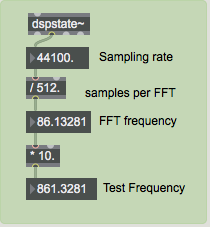
When audio is turned on, dspstate~ sends the MSP sampling rate out its middle outlet. We use this number to calculate a frequency that has a period of exactly 512 samples. This is the fundamental frequency of the FFT itself. If we send a wave of that frequency into fft~, each time slice would contain exactly one cycle of the waveform. We will actually use a cosine wave at ten times that frequency as the test tone for our analysis, as shown below.

The test tone is at 10 times the base frequency of the FFT time slice

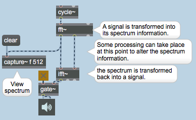
The upper left corner of the Patcher window shows a very simple use of fft~. The analysis is stored in a capture~ object, and an ifft~ object transforms the analysis back into an audio signal. (Ordinarily you would not transform and inverse-transform an audio signal for no reason like this. The ifft~ is used in this patch simply to demonstrate that the analysis-resynthesis process works.)

Click on the toggle in the blue part of the patch to hear the resynthesized sound. Click on the toggle again to close the gate~. Now look at the plot at the bottom of the fft~.

The plot~ shows a single spike at 861.3 Hz. If you click the clear message and double cick the capture~ object, you will see some of the numbers fft~ is putting out. Each of the 512 numbers represents a harmonic of the FFT frequency itself, starting at the 0th harmonic (0 Hz). The analysis shows energy in the eleventh number, which represents the 10th harmonic of the FFT, ¹⁰/₅₁₂ the sampling rate -- precisely our test frequency. The analysis also shows energy at the 10th number from the end, (scroll to see) which represents ⁵⁰²/₅₁₂ the sampling rate. This frequency exceeds the Nyquist rate and is actually equivalent to -¹⁰/₅₁₂ of the sampling rate. (This component is not visible in the plot~ display which is limited to half the sampling rate).

Technical detail: An FFT divides the entire available frequency range into as many bands (often called bins) as there are samples in each time slice. Therefore, each set of 512 numbers coming out of fft~ represents 512 divisions of the frequency range from 0 to the sampling rate. The first number represents the energy at 0 Hz, the second number represents the energy at ¹/₅₁₂ the sampling rate, the third number represents the energy at ²/₅₁₂ the sampling rate, and so on.

Note that once we reach the Nyquist rate on the 257th number (²⁵⁶/₅₁₂ of the sampling rate), all numbers after that are folded**back down from the Nyquist rate. Another way to think of this is that these numbers represent negative frequencies that are now ascending from the (negative) Nyquist rate. Thus, the 258th number is the energy at the Nyquist rate minus¹/₅₁₂ of the sampling rate (which could also be thought of as -²⁵⁵/₅₁₂ the sampling rate). In our example, we see energy in the 11th frequency region (¹⁰/₅₁₂ the sampling rate) and the 503rd frequency region (-²⁵⁶/₅₁₂ - -²⁴⁶/₅₁₂ = -¹⁰/₅₁₂ the sampling rate).

It appears that fft~ has correctly analyzed the signal. There's just one problem...

Practical problems of the FFT

The FFT assumes that the samples being analyzed comprise one cycle of a periodic wave. In our example, the cosine wave was the 10th harmonic of the FFT's fundamental frequency, so it worked fine. In most cases, though, the 512 samples of the FFT will not be precisely one cycle of the wave. When that happens, the FFT still analyzes the 512 samples as if they were one cycle of a waveform, and reports the spectrum of that wave. Such an analysis will contain many spurious frequencies not actually present in the signal.

Close the text window of capture~. With the audio still on, set the ‘Test Frequency’ number box to 1000. This also triggers the clear message in the upper left corner of the patch to empty the capture~ object of its prior contents. Double-click once again on capture~ to see its new contents.

The analysis of the 1000 Hz tone does indeed show greater energy at 1000 Hz -- in the 12th and 13th frequency regions if your MSP sampling rate is 44,100 Hz -- but it also shows energy in virtually every other region. That's because the waveform it analyzed is no longer a sinusoid. (An exact number of cycles does not fit precisely into the 512 samples.) All the other energy shown in this FFT is an artifact of the ‘incorrect’ interpretation of those 512 samples as one period of the correct waveform. Also if you close the capture~ object, hit clear and reopen it, you will see that the numbers have all changed, as the phase relationship between 1000Hz and 947.5 (the 11th harmonic of the fft frequency) will be constantly changing.

All of this will be visible in the plot, which has a broad peak with constantly changing skirts. To resolve this problem, we can try to ‘taper’ the ends of each time slice by applying an amplitude envelope to it, and use overlapping time slices to compensate for the use of the envelope.

Overlapping FFTs

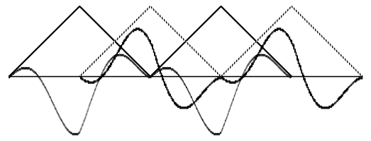
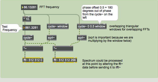
The right portion of the tutorial patch takes this approach of using overlapping time slices, and applies a triangular amplitude envelope to each slice before analyzing it, and again after resynthesizing it. (Other shapes of amplitude envelope are often used for this process, but the triangular window is simple and fairly effective.) In this way, the fft~ object is viewing each time slice through a triangular window which tapers its ends down, thus filtering out many of the false frequencies that would be introduced by discontinuities. This technique is known as windowing.

Overlapping triangular windows (envelopes) applied to a 100 Hz cosine wave

To accomplish this windowing and overlapping of time slices, we must perform two FFTs, one of which is offset 256 samples later than the other. (Note that this part of the patch will only work if your current MSP Signal Vector size is 256 or less, since fft~ can only be offset by a multiple of the vector size.) The offset of an FFT can be given as a (third) typed-in argument to fft~, as is done for the fft~ object on the right. This results in overlapping time slices.

One FFT is taken 256 samples later than the other

The windowing is achieved by multiplying the signal by a triangular waveform (stored in the buffer~ object—double-click to view its contents) which recurs at the same frequency as the FFT -- once every 512 samples. The window is offset by ¹/₂ cycle (256 samples) for the second fft~. Notice also that because we will be applying the amplitude envelope twice (once before the fft~ and once again after the ifft~), we take the square root of the envelope values, so we do not have unwanted amplitude modulation resulting from our envelopes (we want the overlapping envelopes to crossfade evenly and always add up to 1).

Click the toggle labeled Show Windowed Analysis. This will add the windowed fft (in red) to the display.

As with the unwindowed FFT, the energy is greatest around 1000 Hz, but here the (spurious) energy in all the other frequency regions is greatly reduced by comparison with the unwindowed version.

Displaying spectra with plot~

The plot~ object is designed to show graphs of listed data or audio signals. With the latter, it works a lot like scope~, where the portion of waveform shown is determined by the number of points in the display. In plot~ this is set with a numpoints message. plot~ has a lot of options, especially if you want to add gridlines and titles to the display. Luckily, there are some prototypes available for plot~, accessed via the button at the left edge of the display. Prototypes include several spectral displays complete with gridlines and labels.

There is some assembly required before plot can show the fft spectrum. Open the Display_analysis subpatch to see what is required.

The signals from fft~ can reach very high values (as high as the frame size) and must be scaled down to a maximum of 1.0 for plot~. Hence the divide by 512.
The power in each bin is represented by a complex number. The magnitude of a complex number is the square root of the sum of the squares of the real and imaginary parts, so each signal from the fft~ is squared before they are added together. If we leave the square root out, we wind up with an exponential scale, appropriate to show as dB.
Plot~ has no triggering mechanism as scope~ and spectroscope~ do, so the signal from fft~ needs to be stabilized before it can be displayed. The vectral~ object is ideal for this, as it aligns incoming sames with indices in the left inlets. The right outlet of fft~ produces a ramp of bin numbers from 0 to the window size, perfect of vectral~. vectral can also average the values over several frames, which makes the display smoother.

Most of the time, we will use spectroscope~ as our spectral display, but if you want custom features or extra high resolution, plot~ and fft~ allow you to roll your own.

Signal processing using the FFT

In this patch we have used the fft~ object to view and analyze a signal, and to demonstrate the effectiveness of windowing the signal and using overlapping FFTs. However, one could also write a patch that alters the values in the signal coming out of fft~, then sends the altered analysis to ifft~ for resynthesis. This kind of processing using overlapped, windowed time slices is known as a Short Term Fourier Transform (STFT), and is the basis for frequency-domain audio processing. We will be discussing a simpler way to use the STFT in Tutorial 26.

Windowing, in addition to being important for reducing the false frequencies from discontinuities in the input waveform, as we have already seen, is also important to smooth out any discontinuities which occur in the resynthesized time-domain waveform coming from the ifft~. This is why we must window the time-domain signal both on input and output. In this tutorial we would only get such output discontinuities if we modified the signal between the fft~ and ifft~ objects.

Summary

The fast Fourier transform (FFT) is an algorithm for transforming a time-domain digital signal into a frequency-domain representation of the relative amplitude of different frequency regions in the signal. An FFT is computed using a relatively small excerpt of a signal, usually a slice of time 512 or 1024 samples long. To analyze a longer signal, one performs multiple FFTs using consecutive (or overlapping) time slices.

The fft~ object performs an FFT on the signal it receives, and sends out (also in the form of a signal) a frequency-domain analysis of the received signal. The only object that understands the output of fft~ is ifft~ which performs an inverse FFT to synthesize a time-domain signal based on the frequency-domain information. One could alter the signal as it goes from fft~ to ifft~, in order to change the spectrum.

The FFT only works perfectly when analyzing exactly one cycle (or exactly an integer number of cycles) of a tone. To reduce the artifacts produced when this is not the case, one can window the signal being analyzed by applying an amplitude envelope to taper the ends of each time slice. The amplitude envelope can be applied by multiplying the signal by using a cycle~ object to read a windowing function from a buffer~ repeatedly at the same rate as the FFT itself (i.e., once per time slice). To eliminate any artifacts that result from modifying the frequency-domain signal, we must also apply the same envelope at the output of the ifft~.