Tutorial 48: Frames of MSP signals
In Tutorial 27: Using MSP Audio in a Jitter Matrix we learned how to use the jit.poke~ object to copy an MSP audio signal sample-by-sample into a Jitter matrix. This tutorial introduces jit.catch~, another object that moves data from the signal to the matrix domain. We’ll see how to use the jit.graph objects to visualize audio and other one-dimensional data, and how jit.catch~ can be used in a frame-based analysis context. We’ll also meet thejit.release~ object, which moves data from matrices to the signal domain, and see how we can use Jitter objects to process and synthesize sound.
The patch is divided into several smaller subpatches. In the upper left the patcher contains a network labeled Sine wave madness where some cycle~ objects modulate each other. Playback of an audio file is also possible through the sfplay~ object in the upper-right hand corner of the subpatch.
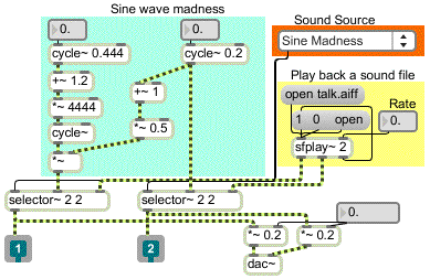
Basic Viz
• Click the message box labeled to begin processing audio vectors.

In the patcher the two signals from the patcher are input into a jit.catch~ object. The basic function of the jit.catch~ object is to move signal data into the domain of Jitter matrices. The object supports the synchronous capture of multiple signals; the object’s first argument sets the number of signal inputs; a separate inlet is created for each. The data from different signals is multiplexed into different planes of a Jitter matrix. In the example in this subpatch, two signals are being captured. As a result, our output matrices will have two planes.
The jit.catch~ object can operate in several different ways, according to the attribute. When the attribute is set to , the object simply outputs all the signal data that has been collected since the last was received. For example, if 1024 samples have been received since the last time the object received a , a one-dimensional cell matrix would be output.
The object’s causes jit.catch~ to output whatever fits in a multiple of a fixed frame size, the length of which can be set with the attribute. The data is arranged in a two dimensional matrix with a width equal to the . For instance, if the were and the same 1024 samples were internally cached waiting to be output, in a would cause a matrix to be output, and the 24 remaining samples would stay in the cache until the next . These 24 samples would be at the beginning of the next output frame as more signal data is received.
When working in , the object outputs the most recent data of length. Using the example above (with a of and 1024 samples captured since our last output), in our jit.catch~ object would output the last samples received.
In our subpatch, our jit.catch~ object is set to use , which causes it to act similarly to an oscilloscope in trigger mode. The object monitors the input data for values that cross a threshold value set by the attribute. This is most useful when looking at periodic waveforms, as we are in this example.
Note that and of the jit.catch~ object attempt to output every signal value received exactly once, whereas and do not. Furthermore, the matrices output in and will be variable in size, whereas those output in and will always have the same dimensionality. For all modes, the jit.catch~ object must maintain a pool of memory to hold the received signal values while they are waiting to be output. By default the object will cache 100 milliseconds of data, but this size can be increased by sending the object a message with an argument of the desired number of milliseconds. In and , when more data is input than can be internally stored, the next will not output a matrix but instead will cause a buffer overrun message to be output from the dump (right-hand) outlet of the object.
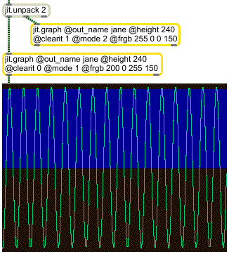
Since the two signals are multiplexed across different planes of the output matrices, we use the jit.unpack object to access the signals independently in the Jitter domain. In this example, each of the resulting single-plane matrices is sent to a jit.graph object. The jit.graph object takes one-dimensional data and expands it into a two-dimensional plot suitable for visualization. The low and high range of the plot can be set with the and attributes, respectively. By default the graph range is from to .
These two jit.graph objects have been instantiated with a number of attribute arguments. First, the attribute has been specified so that both objects render into a matrix named . Second, the right-hand jit.graph object (which will execute first) has its attribute set to , whereas the left-hand jit.graph object has its attribute set to . As you might expect, if the attribute is set to the matrix will be cleared before rendering the graph into it; otherwise the jit.graph object simply renders its graph on top of whatever is already in the matrix. To visualize two or more channels in a single matrix, then, we need to have the first jit.graph object clear the matrix (); the rest of the jit.graph objects should have their attribute set to .
The jit.graph object’s attribute specifies how many pixels high the rendered matrix should be. A attribute is not necessary because the output matrix has the same width as the input matrix. The attribute controls the color of the rendered line as four integer values representing the desired alpha, red, green, and blue values of the line. Finally, the attribute of jit.graph allows four different rendering systems: renders each cell as a point; connects the points into a line; shades the area between each point and the zero-axis; and the bipolar mirrors the shaded area about the zero-axis.
Frames
• Turn off the qmetro (by un-checking the toggle box) and close the subpatch. Open the patcher named and click the toggle box inside to activate the qmetro object.
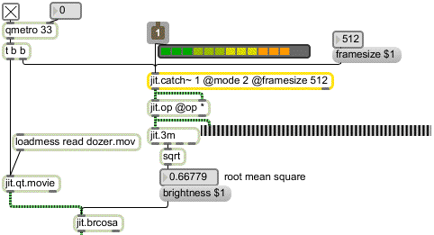
The subpatch shows an example of how one might use the jit.catch~
object’s ability to throw out all but the most recent data. The single-plane output of
jit.catch~ is being sent to a jit.op object which is multiplying it by itself, squaring each
element of the input matrix. This is being sent to a jit.3m object, and the mean value of the
matrix is then sent out the object’s middle outlet to a sqrt object. The result is that we’re
calculating the root mean square (RMS) value of the signal – a standard way to measure
signal strength. Using this value as the argument to the attribute of a jit.brcosa object, our subpatch maps the amplitude of the audio signal to brightness of a video image.
Our frame-based analysis technique gives a good estimate of the average amplitude of the
audio signal over the period of time immediately before the jit.catch~ object received its
most recent . The peakamp~ object, which upon receiving a outputs the highest
signal value reached since the last , can also be used to estimate the amplitude of an
audio signal, but it has a couple of disadvantages compared to the jit.catch~ technique examines only the final 512 samples, thereby striking a balance between accuracy and efficiency. The effect that this savings makes is amplified in situations where the analysis itself is more expensive, for example when performing an FFT analysis on the frame.
• Turn off the qmetro and close the subpatch. Open the patcher named again and enter a into the number box connected to the *~ objects at the bottom of the patch; the generated signals will no longer being sent to your speakers. Close the subpatch and open the patcher named .
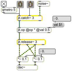
The jit.release~ object is the reverse of jit.catch~: multi-plane matrices are input into the
object which then outputs multiple signals, one for each plane of the incoming matrix.
The jit.release~ object’s attribute controls how much matrix data should be buffered
before the data is output as signals. Given a Jitter network that is supplying a jit.release~
object with data, the longer the the lower the probability that the buffer will
underflow – that is, the event-driven Jitter network will not be able to supply enough data
for the signal vectors that the jit.release~ object must create at a constant (signal-driven) rate.
• Click on the toggle box into the subpatch to start the qmetro object. You should begin to hear our sine waves mixed with white noise (supplied by the noise~ object). Change the value in the number box attached to the message box labeled . Note the effect on the amplitude of the sounds coming from the patch.
The combination of jit.catch~ and jit.release~ allows processing of audio to be
accomplished using Jitter objects. In this simple example a jit.op object sits between the
jit.catch~ and jit.release~ objects, effectively multiplying all three channels of audio by the
same gain. For a more involved example of using jit.catch~ and jit.release~ for the
processing of audio, look at the jit.forbidden-planet example, which does frame-based FFT processing in Jitter.
Varispeed
The jit.release~ object can operate in one of two modes: in the standard it expects
that it will be supplied directly with samples at the audio rate – that is, for CD-quality
audio the object will on average receive 44,100 elements every second and it will
place those samples directly into the signals. In , however, the object will interpolate
in its internal buffer based on how many samples it has stored. If the playback time of
samples stored is less than the length of the latency attribute, jit.release~ will play through
the samples more slowly. If the object stops receiving data altogether, playback will slide
to a stop in a manner analogous to hitting a turntable platter’s stop button. On the other
hand, if there are more samples than needed in the internal buffer, jit.release~ will play through the samples more quickly.
One can use this feature to generate sound directly from an event-driven network. The
subpatch shows a way for us to do this. The data that drives the
jit.release~ object in this subpatcher receives data from a jit.buffer~ object, which allows us
to extract data from audio samples in matrix form using messages to the MSP buffer~
object. The jit.buffer~ object is essentially a Jitter wrapper around a regular buffer~ object;
jit.buffer~ will accept every message that buffer~ accepts, allows the getting and setting
of buffer~ data in matrix form, and also provides some efficient functions for visualizing
waveform data in two dimensions, which we use in this patch in the jit.pwindow object at
right. At loadbang time this jit.buffer~ object loaded the data in the sound file .
• Turn on the toggle box connected to the qmetro object in the subpatch. Play with the number boxes labeled period and length ratio and the slider object labeled start.
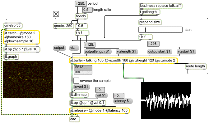
The rate of the qmetro determines how often data from the jit.buffer~ object is sent down towards the jit.release~ object. The construction at the top maintains a ratio between the period and the number of samples that are output from jit.buffer~. Experimenting with the start point, the length ratio, and the output period will give you a sense of the types of sounds that are possible in this of jit.release~.
Summary
In this Tutorial we were introduced to jit.catch~, jit.graph, jit.release~, and jit.buffer~ as objects for storing, visualizing, outputting, and reading MSP signal data as Jitter matrices. The jit.catch~ and jit.release~ objects allow us to transform MSP signals into Jitter matrices at an event rate, and vice versa. The jit.graph object provides a number of ways to visualize single-dimension matrix data in a two-dimensional plot, making it ideal for the visualization of audio data. The jit.buffer~ object acts in a similar manner to the MSP buffer~ object, allowing us to load audio data directly into a Jitter matrix from a sound file.
See Also
| Name | Description |
|---|---|
| jit.3m | Report min/mean/max values |
| jit.brcosa | Adjust image brightness/contrast/saturation |
| jit.buffer~ | A matrix-friendly MSP buffer~ |
| jit.catch~ | Transforms signal data into matrices |
| jit.graph | Floating-point data visualization |
| jit.op | Apply binary or unary operators |
| jit.qt.movie | Play or edit a QuickTime movie |
| jit.release~ | Transforms matrix data into signals |