Tutorial 12: Color Lookup Tables
In this tutorial we will explore how to use color lookup tables to remap data inside a Jitter matrix. The jit.charmap object is a powerful tool for this. We'll also look at different strategies for generating matrices to use as lookup tables, including the jit.gradient object.
The lookup process
Lookup tables (which are often called transfer functions) are arrays of numbers where an input number is used as an index in the table. The number stored at that index (or address, or position) is then retreived to replace the original number. Any function—a graph where each x value (address) has a corresponding y value (output)—can be used as a lookup table. Max objects such as funbuff, table, and the MSP buffer~ object are common candidates for use as lookup tables. In this tutorial, we'll be using Jitter matrices in much the same way.
- Open the tutorial patch.
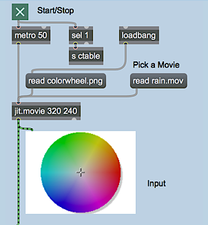
The top left of the patch shows a jit.movie object in which you can read two different files. The object is initialized (via loadbang) with the file colorwheel.pct loaded into it. You can also load in the movie rain.mov by clicking on the message box that says read rain.mov. You should feel free to alternate between the two image sources throughout the tutorial.
- Start the metro by clicking the toggle box at the top of the patch. You will see the color wheel appear in both the jit.pwindow at the top and the jit.pwindow at the bottom of the patch. In addition, you will see a gradient appear in a third (rectangular) jit.pwindow at the bottom.
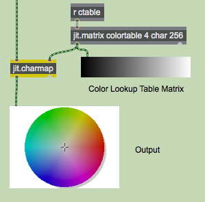
The bottom of the patch contains a jit.charmap object, which we will use in this tutorial to remap cell values in the image. The object has two inlets, the left one of which is connected to our jit.movie object at the top of the patch. The right inlet is connected to a jit.matrix named colortable. The colortable matrix is one-dimensional, with four planes of char and a width of 256 cells. This is the lookup table that jit.charmap uses to remap the color values of the cells in the lefthand matrix. The receive object (abbreviated r) with the name ctable receives data from elsewhere in the patch and sends it to the jit.matrix. For example, turning on the toggle box at the top of the patch will send a bang to the colortablejit.matrix, causing it to send its matrix message to both the jit.pwindow and jit.charmap.
The jit.charmap object builds its output matrix by using the values in the input (left) matrix to point to positions in the (right) matrix and copying the value found there. For example, assume that the matrix we send to jit.charmap contains a cell with the values 100 50 35 20 in its four planes. If our lookup table has the value 73 at cell 100 in the first plane, 25 at cell 50 in the second plane, 0 at cell 35 in the third plane, and 203 at cell 20 in the fourth plane, our output cell will contain the values 73 25 0 203.
Lookup tables for jit.charmap should be one-dimensional matrices of 256 cells with the same number of planes as the matrix you want to remap. This is because the possible range of values for char matrices is 0-255, so 256 numbers are need to cover the full range of the lookup table.
Generating the Lookup Table
The upper-right side of the tutorial patch contains three multislider objects that let you design the transfer functions for planes 1-3 of the lookup table matrix colortable :
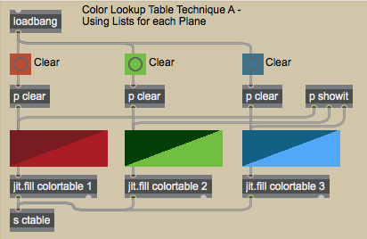
The multislider objects (which have 256 integer sliders in the range 0-255) send their lists to the jit.fill objects below them. These objects replace the values currently stored in planes 1-3 (i.e. Red, Green, and Blue) of the matrix colortable with the values from the multislider objects. (See Tutorial 11.) When the matrix has been edited with the new values, the jit.fill objects send out a bang, which we send to the jit.matrix on the right of the patch that connects to the right inlet of jit.charmap. We're ignoring plane 0 in this tutorial because it only contains Alpha values when we treat 4-plane Jitter matrices as video.
The jit.matrix and jit.fill objects in our patch share the same name (colortable). As a result, the two objects read from and write to the same matrix, allowing one object (jit.fill) to generate data that the other object (jit.matrix) can read from without having to copy data between two separate matrices. This is similar to how many MSP objects (e.g. peek~, play~, groove~) can share sample data stored in a single buffer~. See Tutorials 11, 16, and 17 for more information on using named matrices.
- Do some freehand drawing in the multislider objects, to see how this affects both the lookup table (the smaller of the jit.pwindow objects) and the output image from the jit.movie object. Remember to switch back and forth between the two image sources.
If you want to reset any of the planes to a y="x" transfer function (i.e. a straight ascending line that leaves all the values unchanged), you can click the button object above the relevant multislider object. The subpatchers called pclear initialize the multislider objects with an uzi.
Important note: Like many Max objects, Jitter objects retain matrices stored in one inlet even if a new matrix arrives in another inlet. The metro object in this patch, therefore, only needs to trigger the jit.movie object. The jit.matrix that contains the lookup table to jit.charmap only needs to output its value to the object when the data stored in it actually changes.
Here are some lookup tables and their results:

In the first example, the red and blue transfer functions are approximately inverted while the green is normal. The result is that high values of red and blue in the input image yield low values on the output, and vice versa. This is why the white background of the color wheel now looks green (the cell values of 0 255 255 255 have been mapped to 0 0 255 0).
The second example has the green plane completely zeroed (the transfer function set to 0 across the entire span of input values). The red and blue planes are also set to 0 up to a threshold, at which point they ramp up suddenly (the red more suddenly than the blue). As a result the majority of the colorwheel is black (especially in the 'green' area). The red plane only becomes visible in very high values (i.e. the magenta in the background of the color wheel).
The third example has the red plane mapped normally. The green plane has a parabolic shape to it, where the extreme values are mapped high and the medium shades are mapped low. The blue plane is normal except for a range in the midtones, where it is zeroed. This nonlinearity is visible as a red 'fault line' across the top and down the right side of the colorwheel.
As you can see, there are infinite ways to remap the cell values of these matrices. We'll now investigate another object, which lets us remap the color values in a more precise manner.
The jit.gradient object
- Open the
Duotonesubpatch
This subpatch shows a method for generating lookup tables using the jit.gradient object:
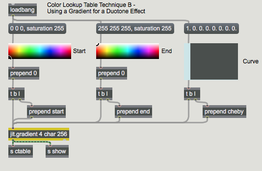
The jit.gradient object generates single dimension char matrices that transition smoothly between two specified cell values. The start and end attributes are lists that specify these cell values. For example, a start attribute of 0 0 0 0 and an end attribute of 0 0.5 1.0 0.5 will generate a gradient that goes from black (at cell 0 in the matrix) to pale green (at the last cell in the matrix). We've given our jit.gradient object the relevant arguments to make it 256 cells wide, so that it can be stored in our colortablejit.matrix when it changes. Note that jit.gradient takes floating point numbers in its attribute lists to specify char values (i.e. a value of 1.0 in the attribute specifies a char value of 255).
The attributes are formatted by taking the RGB list output of the Max swatch objects and converting them to ARGB floats. After the attribute has been sent to the jit.gradient object, the object is given a bang from the trigger object to cause it to output its matrix into the jit.matrix object on the left of the patch.
- Try selecting some colors in the swatch objects. The
startandendattributes will specify the boundaries of the lookup table, so values in the input image will have a duotone appearance, morphing between those two colors. The multislider objects at the top of the patch will reflect the correct lookup tables generated by the jit.gradient object.
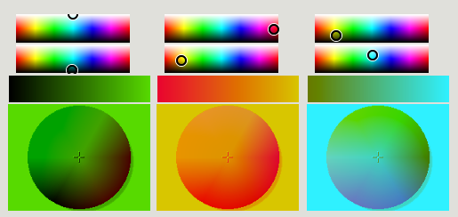
The first example shows an inverted image. The start of the lookup table is white (start 0 1.0 1.0 1.0) and the end of the lookup table is black (end 0. 0. 0. 0.). As a result, input values of 0 are mapped to 255, and vice versa (y=255-x).
The second and third examples show duotone gradients that remap the color wheel's spectrum to between red and orange (example 2) and olive and cyan (example 3). Notice how, depending on the original colors at different points in the color wheel, the gradient curve becomes steeper or more gradual.
The third attribute of the jit.gradient object is the cheby attribute, which specifies a curve to follow when morphing between the start and end values in the matrix. The cheby attribute takes a list of floating point numbers as arguments. These arguments are the amplitudes of different orders of Chebyshev polynomials (see below). These special function curves create different effects when used in lookup tables. The multislider in the tutorial patch that sets the cheby attribute lets you specify the relative amplitude of the first eight Chebyshev polynomial curves, which have the following shapes (if you view them as progressing from black to white):

Technical note: Chebyshev polynomials are commonly used as transfer functions in waveshaping audio signals in digital synthesis algorithms (they have special properties that allow them to distort sinusoidal waveforms into harmonic spectra equivalent to the amplitudes of different orders). The MSP lookup~ object can be used with a function loaded into a buffer~ to do the equivalent process in audio signal processing that we're doing in this tutorial with image. See Tutorial 12: Synthesis: Waveshaping in the MSP manual for more details.
- Reset the
startandendpoints of the gradient (by clicking the message boxes above them) and slowly change the multislider that controls thechebyattribute. Watch how the color wheel changes as colors disappear and reappear in different regions.
When you use the cheby attribute in the jit.gradient object, you can get some very interesting color warping effects even if you leave the start and end points of the gradient at black and white. Here are some examples with our movie clip rain.mov :
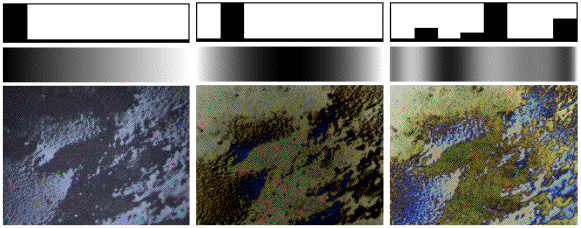
The lefthand image shows an unprocessed still image from the rain movie. The middle image shows what happens to the color spectrum when the gradient is generated using a second order Chebyshev polynomial (the darkest area in the image is now in the middle of the color spectrum). The righthand image shows a more complex gradient, where the color spectrum shows numerous peaks and troughs.
- The multislider objects at the top of the patch reflect the current state of our lookup table (the matrix generated by our jit.gradient object is sent to a jit.iter object inside of the p
showitsubpatch, where the numbers are grouped to set the state of the multislider objects). Try generating a gradient and then modifying the lookup table by hand by changing the multislider objects. This lets you use the jit.gradient object as a starting point for a more complicated lookup table.
Summary
You can map cell values in char Jitter matrices using the jit.charmap object. The right inlet of jit.charmap takes a 256 -cell matrix that defines the lookup table (or transfer function) to be applied to the incoming matrix data. You can define the lookup table using several strategies, including using jit.fill to generate the matrix from Max lists, or using the jit.gradient object to generate color gradients between a start and end cell value according to a curve shape specified by the cheby attribute.